Empowered AI¶

Empowered AI is a module of ITRS Log Analytics containing mathematical algorithms for data science. It is a licensed extension for SIEM deployment, designed to help SOC teams detect data that is difficult to identify with regular approaches. Advanced mathematical sorting, grouping, and forecasting enriched with statistics create a new outlook on security posture.

Empowered AI is an ongoing project, continuously improved by a team of mathematicians, data scientists, and security analysts.

Table of Contents¶

Empowered AI

AI Rules¶

In the Empowered AI section you will find a summary of the existing rules. At the top, you’ll find the total number of rules and the number of scheduled and unscheduled rules. Here is the search field and buttons Refresh rules list and Create New Rule, below is the table. It contains AI Rule Name, Search/Index Name - data source, Last Executed - date, Last Modified - date, selected Use Case, Schedule - scheduling frequency, Status and Action icons.

../_images/rule_table1.png

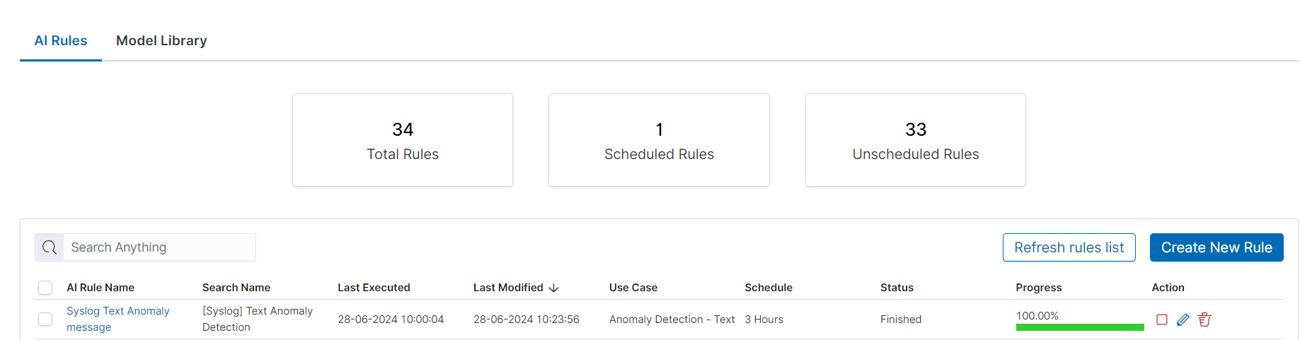
Status¶

The rule has one of the following statuses:

Waiting to start - Run once rule starts by clicking symbol play.
Scheduled - the scheduled rule starts automatically.
Scoring
Building
Finished - click on the AI Rule Name to get the forecast results preview AI Rules>Performance.
Error - check error details in the results preview Performance>AI Rules>Performance>Exceptions.

Actions¶

Icons of actions:

Play – run or rerun the rule,
Stop – unschedule periodic rule, after this action rule type changes to Run Once,
Pencil - edit the rule’s configuration,
Bin – delete the rule.

Common Elements¶

Settings and Configuration for all Analytical Use Cases¶

The first step in the data analysis process in the Empowered AI module is to properly prepare the data and input it into an analytical rule using saved searches as data sources.

Log in to the application and access the Discover module.
Select the data source you want to analyze (e.g., system logs, application records).
Set filters and search criteria to narrow down relevant data (kql/oql not supported).
Add a field as a column, which allows selecting the field during rule creation.

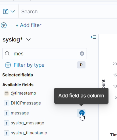AddFieldAsColumn
Save the search by clicking the Save button, naming your search, and clicking Save again.

CreateSavedSearch

Defining Data Source in the Empowered AI Module¶

Go to the Empowered AI module.

GoToEmpoweredAIModule
Select the AI Rules tab and click Create New Rule or edit an existing rule.
In the Choose Data Source section, select the saved search you created earlier.

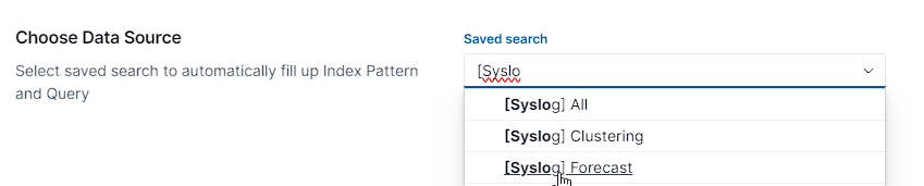SelectSavedSearch
After selection Index Pattern and query will be automaticly filled up based on saved search. Alternatyivly you can skip saved search and fill up index pattern and query by yourself.

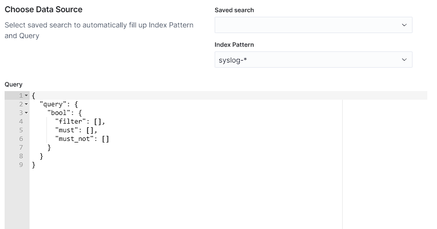IndexPatternAndQuery
Time Field will be fetched automatically from your Index Pattern. TimeField

Configuring the Analytical Rule¶

Name your rule in the AI Rule Name section.
In the Field to Analyse section, select the data field you want to analyze.

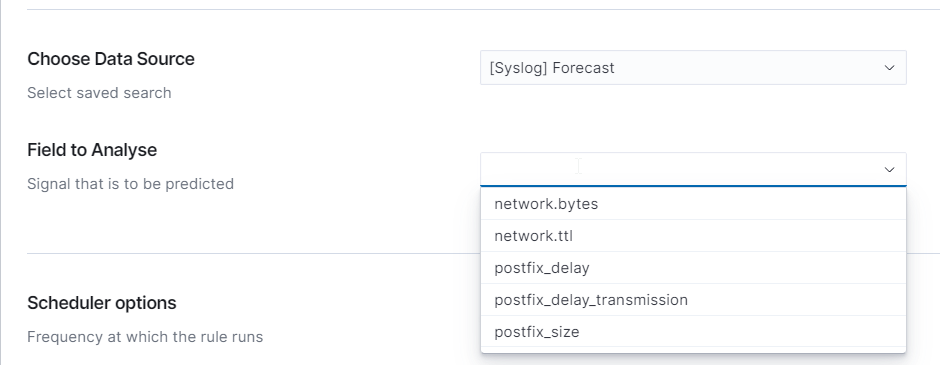ConfigureRule

Configuring the Scheduler¶

The rule can be run immediately using the Run Once option or cyclically using the Scheduled option.

For Run Once analysis, provide the “Build Time Frame” learning period and the analysis start time using the trained model “Start Date”.

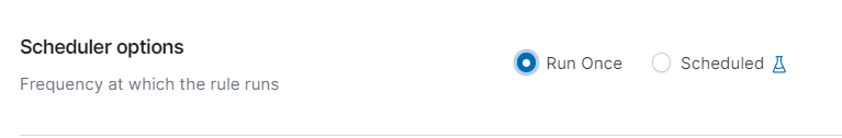RunOnce 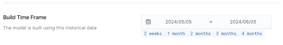BuildTimeFrame StartDate
For Scheduled analysis, choose the run frequency (e.g., every hour, day, week, or month). Specify the learning period and the “Start Date Offset” for the data range to be analyzed.

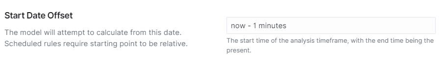StartDateOffset
Actual Log Count: Displays the number of logs to be analyzed.

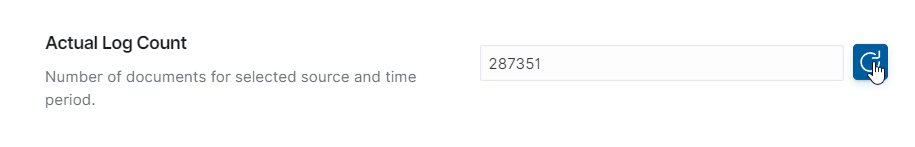ActualLogCount

Accessing the Performance Tab¶

Log in to the application and navigate to the Empowered AI module.
Select the AI Rules tab and click on the rule for which you want to view the performance.
The Performance tab will open, displaying detailed analysis results.

Summary¶

This basic configuration is common to all analytical models. Some models require additional parameters, detailed in their dedicated documentation.

Univariate Anomaly Detection¶

Univariate Anomaly Detection identifies anomalies in a single data column. Below is a guide on configuring Univariate Anomaly Detection, highlighting its unique settings.

Step 1: Configuring the Univariate Anomaly Detection Rule¶

Contamination Factor: This setting defines the approximate percentage of data considered anomalous. The suggested value lower than 5%.

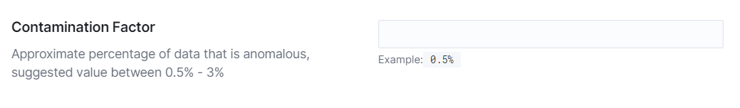ContaminationFactor
Data Aggregation: Select the aggregation interval to be used for training the model. Available intervals are 30 minutes, 1 hour, 2 hours, 4 hours, 8 hours, 12 hours, and 1 day.

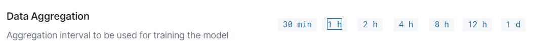DataAggregation
Complete the configuration of other settings, such as Start Date, Build Time Frame, Scheduler options, and Field to Analyse. These settings are the same as those described in the common configuration guide.

Step 2: Running the Rule¶

After configuring all settings, click Save to save the rule, then click Run to start the anomaly detection process or Save & Run to start process imidietly.

Summary¶

Configuring Univariate Anomaly Detection in the Empowered AI module involves setting the contamination factor and selecting the data aggregation interval.

Performance Tab for Univariate Anomaly Detection¶

The Performance Tab provides a visual representation of the model’s performance, particularly focusing on the detected anomalies in a single data column over time.

Understanding the Performance Graph¶

The performance graph displays the actual values of the monitored data and highlights detected anomalies. The x-axis represents the timeline, while the y-axis shows the values of the selected data field, such as netflow.bytes in the given example.

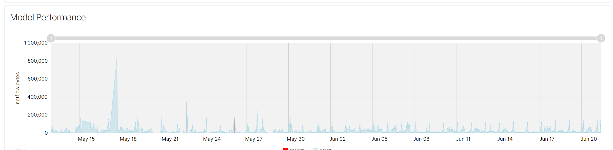../_images/model_performance_graph1.png ModelPerformanceGraph

Key Elements of the Performance Graph¶

Actual Values (Blue Line)
- The blue line represents the actual values of the monitored data over time. This line helps in visualizing the normal behavior of the data and identifying patterns or trends.
Anomalies (Red Markers)
- Red markers indicate the points where anomalies have been detected. These markers are overlaid on the blue line, showing the specific times when the data deviated from the normal pattern.

Interpreting the Graph¶

Spikes and Drops: Significant spikes or drops in the blue line could indicate unusual activity or anomalies in the data. Red markers on these spikes or drops confirm the detection of anomalies by the model.
Consistency: Consistent patterns in the blue line without red markers suggest stable data behavior with no detected anomalies.

Using the Performance Graph¶

Monitoring Trends: The graph allows you to monitor trends and identify periods of abnormal activity.
Investigating Anomalies: By examining the red markers, you can investigate the corresponding timestamps to understand the context of the anomalies.
Adjusting Parameters: If too many or too few anomalies are detected, consider adjusting the contamination factor or other model parameters to improve detection accuracy.

Summary¶

The performance graph in the Performance Tab of the Univariate Anomaly Detection use case provides a clear visual representation of data behavior and detected anomalies over time. By understanding and utilizing this graph, users can effectively monitor and investigate anomalies, ensuring better data analysis and system optimization.

Multivariate Anomaly Detection¶

Multivariate Anomaly Detection identifies anomalies across multiple data columns. Below is a guide on configuring this use case.

Step 1: Configuring the Multivariate Anomaly Detection Rule¶

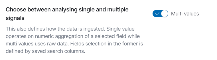
Choose Between Analyzing Single and Multiple Signals

Multi Values: Ensure the toggle for analyzing multiple signals is enabled. This setting defines how the data is ingested. Single value analysis operates on the numeric aggregation of a selected field, while multi-value analysis uses raw data. Field selection in the former is defined by saved search columns.

../_images/multi_values1.png MultiValues

Contamination Factor: This setting defines the approximate percentage of data that is considered anomalous.The suggested value lower than 5%.

../_images/contamination_factor1.png ContaminationFactor

Complete the configuration of other settings, such as Start Date, Build Time Frame, Scheduler options, and Field to Analyse. These settings are the same as those described in the common configuration guide.

Step 2: Running the Rule¶

After configuring all settings, click Save to save the rule, then click Run to start the anomaly detection process or Save & Run to start process imidietly.

Summary¶

Configuring multivariate anomaly detection in the Empowered AI module involves setting the contamination factor and ensuring the analysis mode is set to multi-values.

Performance Tab for Multivariate Anomaly Detection¶

The Performance Tab provides comprehensive visualizations and detailed information on detected anomalies over time.

Visualizing Anomalies Over Time¶

Anomalies Over Time Chart: Displays detected anomalies over time. The X-axis represents time, while the Y-axis represents the anomaly score. Each red vertical line indicates an anomaly detected by the model at a specific time. This visualization helps in identifying periods of high anomaly activity.

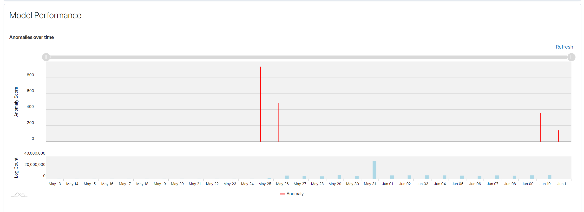Anomalies Over Time
Spread of Anomalies Chart: Shows the distribution of anomaly scores across the entire dataset. Each dot represents an anomaly score, and this chart helps to understand the spread and severity of anomalies in the data.

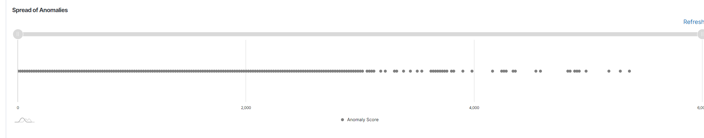Spread of Anomalies
List of Anomalies: Below the charts is a detailed table listing the detected anomalies. The table includes the following columns:
- Time: Timestamp of the detected anomaly.
- Anomaly Score: Score indicating the severity of the anomaly.
- Network.bytes: Specific field from the data that might have contributed to the anomaly.
- Source: Additional context or source information about the anomaly.
This table allows users to review anomaly details and gain insights into specific instances of unusual behavior.

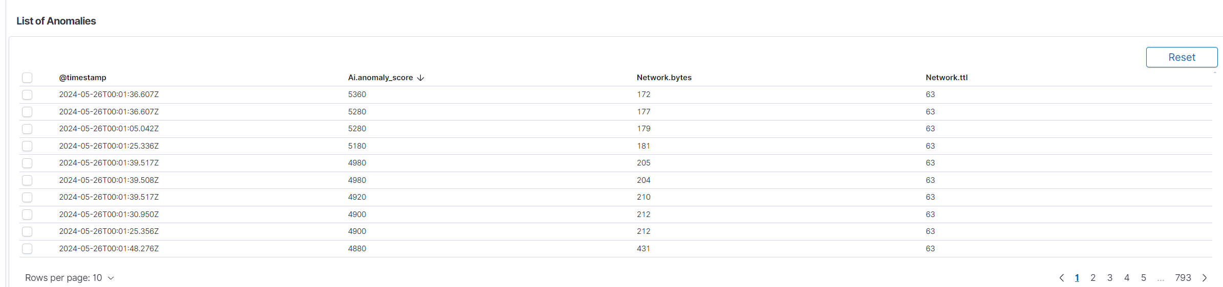List of Anomalies

Summary¶

The performance tab for multivariate anomaly detection in the Empowered AI module provides critical information about anomalies detected by the model. Various charts and tables allow users to visualize anomalies over time, understand their distribution, and review detailed information about each detected anomaly. Correct interpretation of these visualizations is crucial for effectively leveraging anomaly detection capabilities.

Clustering¶

Clustering groups similar data into clusters. Below is a guide on configuring clustering in the Empowered AI module.

Step 1: Configuring the Clustering Rule¶

Number of clusters

In the Clusters section, specify the number of clusters to be created. This number depends on the nature of your data and the objectives of your analysis.

../_images/clusters1.png Clusters

Complete the configuration of other settings, such as Start Date, Build Time Frame, Scheduler options, and Field to Analyse. These settings are the same as those described in the common configuration guide.

Step 2: Running the Rule¶

After configuring all settings, click Save to save the rule, then click Run to start the clustering process or Save & Run to start process imidietly.

Summary¶

Configuring clustering in the Empowered AI module is a straightforward process that involves setting the number of clusters and preparing the appropriate data.

Performance Tab for Clustering¶

The Performance Tab provides comprehensive visualizations and detailed information on clustering results.

Elbow Method and Optimal Number of Clusters¶

The elbow method is a commonly used technique in clustering analysis to determine the optimal number of clusters. It involves plotting cluster quality against the number of clusters and identifying the point where the quality improvement slows down, forming an “elbow” shape on the graph. This point indicates the optimal number of clusters.

Cluster Quality Chart¶

The Cluster Quality Chart visualizes the relationship between the number of clusters and the cluster quality. The x-axis represents the number of clusters, and the y-axis represents the cluster quality score. The goal is to identify the point where adding more clusters does not significantly improve quality, which is the optimal number of clusters.

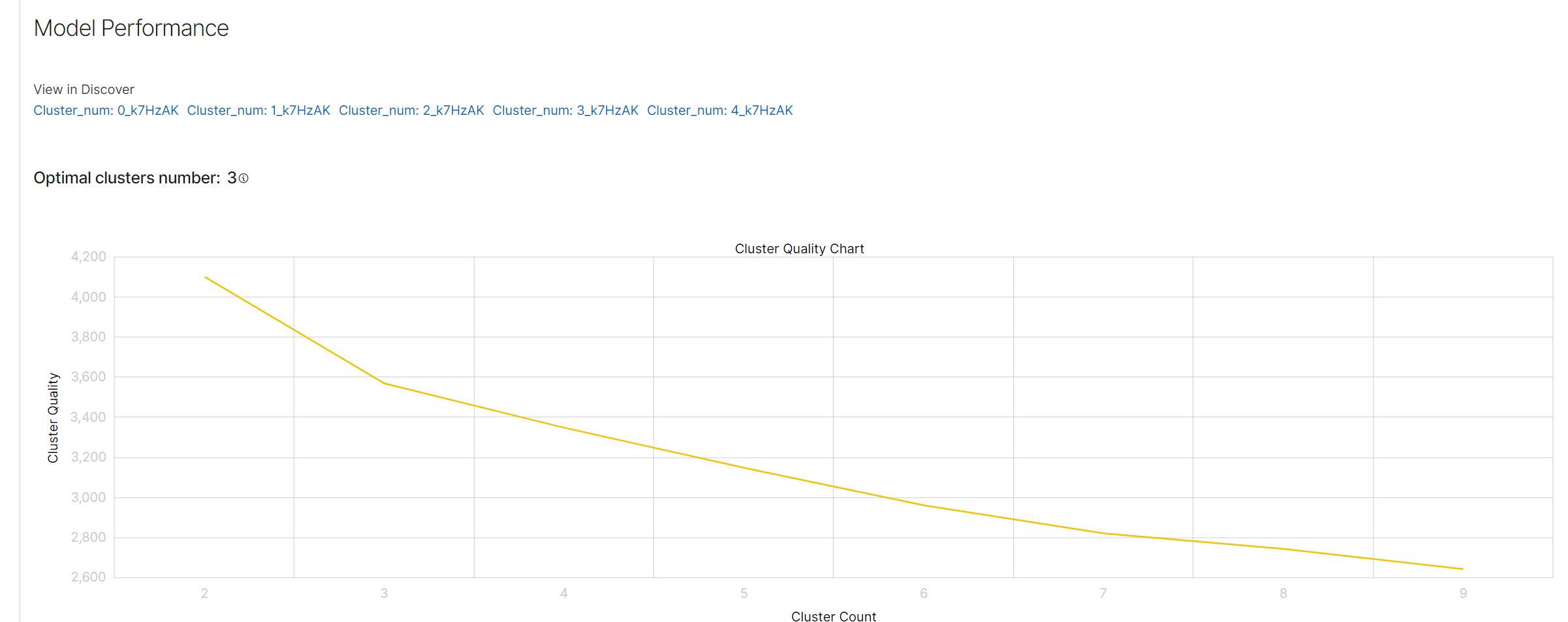../_images/cluster_quality_chart1.png Cluster Quality Chart

In this example, the optimal number of clusters is 3, as indicated on the chart.

Cluster Distribution Chart¶

Below the elbow method chart in the Performance tab, there is a cluster distribution chart. This chart shows the distribution of documents among clusters along with their centers. Each dot on the chart represents a document assigned to a specific cluster.

Clicking on a Dot: Clicking on any dot on the chart will display a preview of the document it represents. The preview contains detailed information about the document, such as the message content.

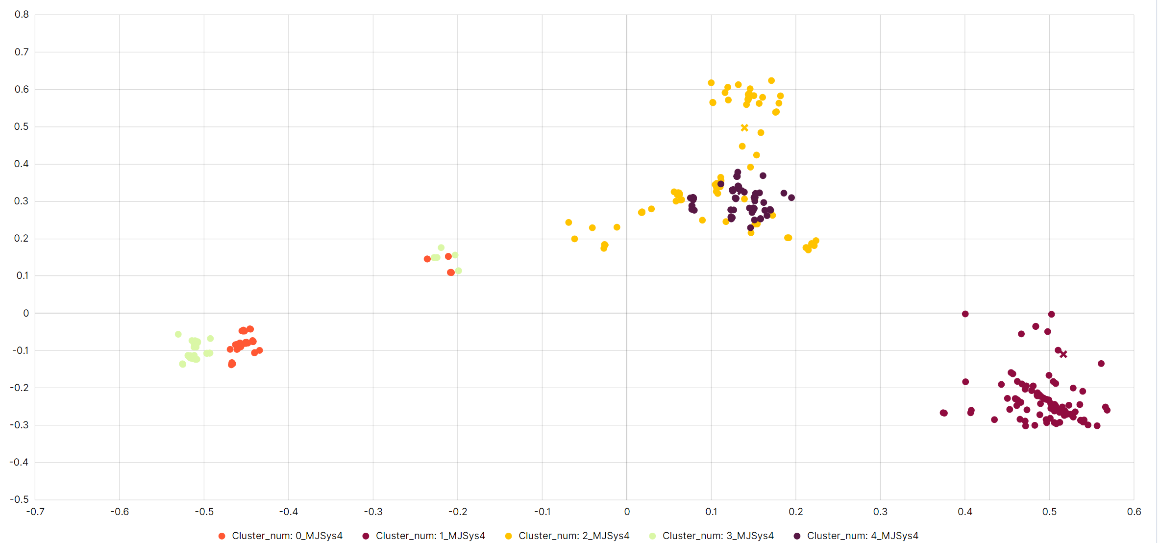../_images/cluster_distribution_chart1.png ClusterDistributionChart

Indicative Number of Documents: The chart shows an indicative number of documents, meaning it does not display the entire dataset. This is done to avoid overcrowding the chart and to provide better readability and data analysis.

Benefits of the Cluster Distribution Chart¶

The cluster distribution chart helps in:

Visualizing Document Groupings: It enables understanding how documents are grouped into clusters and their distributions.
Quick Anomaly Identification: By analyzing the document distribution, unusual groupings can be quickly identified, which may indicate anomalies.
Analyzing Cluster Centers: Cluster centers help evaluate which features are most representative of a given cluster.

Clustering Result Examples¶

Below the cluster distribution chart, the Performance tab displays example documents from each cluster. These documents correspond to the dots on the chart and are not a full set but a representative sample.

Understanding the Clustering Result Examples¶

Document Representation: Each cluster section shows a list of example documents that belong to that cluster. The documents are represented by their content, such as log messages or text data.

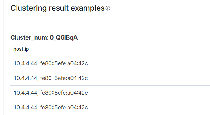ClusteringResultExamples
Sample Data: The documents shown are not exhaustive. Only a sample is displayed to give an idea of the type of data grouped into each cluster. This helps in understanding the nature and characteristics of the clusters without overwhelming the user with too much data.

Benefits of Viewing Clustering Result Examples¶

The clustering result examples help in:

Validating Cluster Quality: By looking at the example documents, you can quickly assess whether the clustering algorithm has grouped the documents meaningfully.
Identifying Patterns: Seeing sample documents from each cluster allows you to identify common patterns or features within each cluster.
Quick Reference: The representative samples provide a quick reference to the kinds of documents in each cluster, aiding in faster analysis and decision-making.

Summary¶

The Performance Tab for clustering in the Empowered AI module is a powerful tool for evaluating clustering analysis results. By using the elbow method and the Cluster Quality Chart, users can determine the optimal number of clusters for their data. Additionally, the ability to view clusters in the Discover module allows for a detailed examination of the data points in each cluster.

Proper use of the Performance tab for clustering analysis in the Empowered AI module is crucial for effective data grouping and system optimization. Use this guide to fully leverage the capabilities of this functionality.

Forecasting¶

Forecasting involves setting the data aggregation interval and the forecast time frame.

Step 1: Data Aggregation¶

Data Aggregation: Select the aggregation interval to be used for training the model. Available intervals are 30 minutes, 1 hour, 2 hours, 4 hours, 8 hours, 12 hours, and 1 day. This setting defines how the data will be grouped over time to build the forecasting model.

Data Aggregation

Step 2: Forecast Time Frame¶

Forecast Time Frame: Choose the future time period for which the model will attempt to predict values. Available options are 4 hours, 8 hours, 12 hours, 1 day, 2 days, 3 days, 1 week, and 1 month. This setting determines the period for which the model’s forecasts will be applied.

Forecast Time Frame

Summary¶

Configuring forecasting in the Empowered AI module involves setting the data aggregation interval and the forecast time frame. Correct configuration of these settings ensures that the model is trained on appropriately grouped data and that forecasts are made for the desired future period.

Performance Tab for Forecasting¶

The Performance Tab provides detailed visualizations and insights into the accuracy and effectiveness of the forecasting model over time.

Forecast vs Actual Data Chart¶

Forecast vs Actual Data Chart: This chart shows forecasted data compared to actual data over time. The chart uses different colors to distinguish between forecasted data (purple) and actual data (yellow).

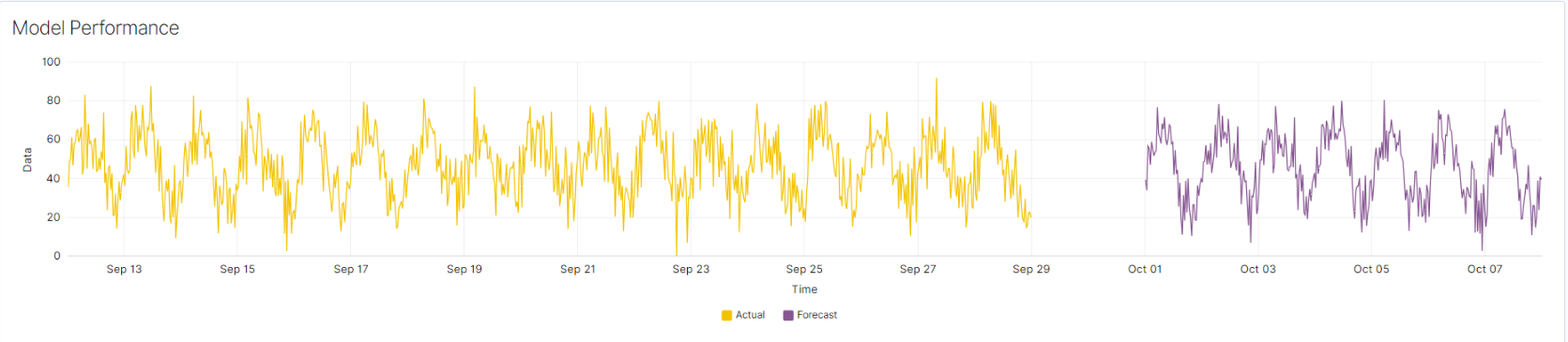ForecastVsActual

Performance Analysis Over Time¶

The performance tab allows users to scroll and zoom in on the timeline to closely examine specific periods where the forecasting model performed well or poorly. This can help identify patterns or anomalies that may affect the forecast’s accuracy.

Summary¶

The performance tab for forecasting in the Empowered AI module provides crucial insights into the accuracy and performance of the forecasting model. Various charts and metrics allow users to visualize forecast accuracy over time, compare predicted values with actual data, and gain insights into the model’s reliability. Proper interpretation of these visualizations is essential for effectively utilizing forecasting capabilities.

Text Anomaly Detection¶

Text Anomaly Detection focuses on analyzing textual data for anomalies.

Key Features¶

Create Alert: Automatically create alert rules for detected anomalies.
Default Text Anomaly Detection Rules: Automatically apply default rules for text anomaly detection at startup.
Exclude Pattern & Words: Exclude specific patterns or words from the analysis.
Performance Tab: Monitor and evaluate model performance.
Rareness Threshold: Set the threshold for word rarity in analyzed documents.
Sampling Rate: Control the percentage of sampled documents for analysis.
Skipping Numerical Values: Automatically skip irrelevant numerical data during analysis.

Create Alert: Automatically create alerts for detected anomalies.

../_images/create_alert1.png CreateAlert

Exclude Pattern & Words: Define patterns and words to be excluded from the analysis.

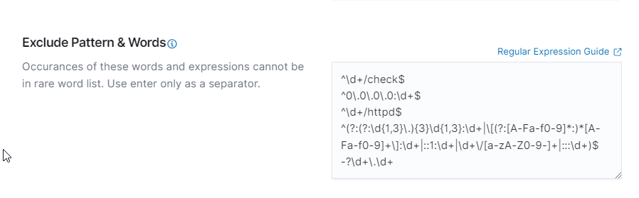../_images/exclude_pattern_and_words1.png ExcludePatternAndWords

Rareness Threshold: Set thresholds for detecting rare words.

../_images/configure_rareness_threshold1.png RarenessThreshold

Sampling Rate: Adjust the percentage of documents to be sampled for analysis.

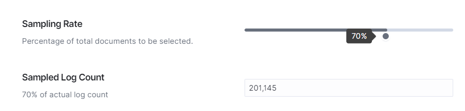../_images/configure_sampling_rate1.png SamplingRate

Skipping Numerical Values: Skip irrelevant numerical data during analysis.

../_images/activate_skip_numbers1.png SkippingNumbers

Summary¶

The Text Anomaly Detection feature in the Empowered AI module offers robust tools for analyzing textual data to identify anomalies. Key features include the ability to create alerts automatically for detected anomalies, and apply default rules at startup. Users can exclude specific patterns and words from the analysis, set thresholds for detecting rare words, control the sampling rate of documents, and skip irrelevant numerical values during analysis.

Proper configuration and utilization of these features enable effective monitoring and detection of anomalies in textual data, enhancing overall security posture.

Performance Tab for Text Anomaly Detection¶

Understanding the Performance Graphs¶

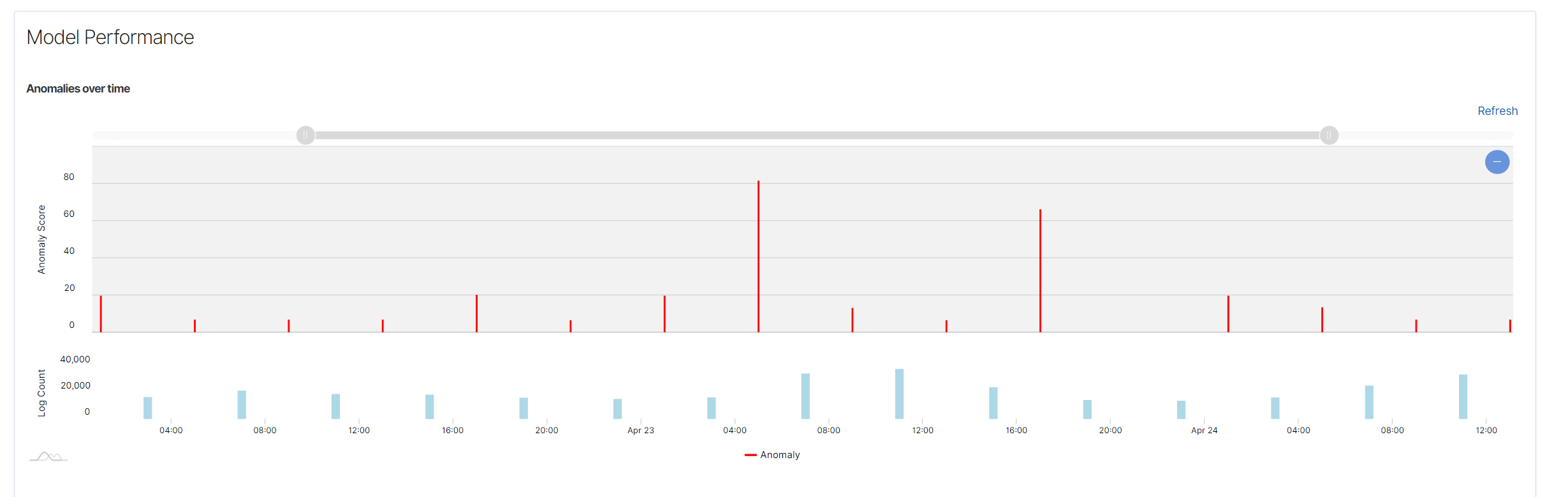../_images/model_performance_graphs1.png ModelPerformance

Anomalies Over Time Chart: Displays detected anomalies over time. The X-axis represents time, while the Y-axis represents the number of detected anomalies.
Spread of Anomalies Chart: Shows the distribution of detected anomalies across the dataset. Each dot represents an anomaly score.

Using the Performance Graphs¶

Monitoring Trends: Allows you to monitor trends and identify periods of abnormal activity.
Investigating Anomalies: By examining the anomaly markers, you can investigate the corresponding timestamps to understand the context.
Adjusting Parameters: If too many or too few anomalies are detected, consider adjusting the rareness threshold or sampling rate.

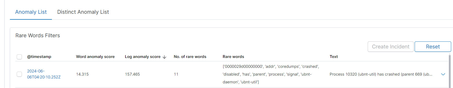
Anomaly Detection Table¶

At the bottom of the Performance tab, there is an anomaly detection table that provides detailed information about each detected case.

Anomaly Detection Table ../_images/anomaly_table1.png AnomalyDetectionTable

Information in the Anomaly Detection Table:¶

@timestamp: The timestamp when the anomaly was detected.
Word anomaly score: The anomaly score for the word, indicating the level of atypicality.
Log anomaly score: The anomaly score for the entire log.
No. of rare words: The number of rare words detected in the log.
Rare words: The list of rare words detected in the log.
Text: A fragment of the text containing the detected anomalies.

Expanding a Row¶

Click the arrow icon next to a specific row to expand detailed information about the anomaly. After expanding the row, you will see the full text containing the anomaly and the list of rare words that have been identified.

../_images/expand_row1.png ExpandingRow

Filtering by Rare Words¶

At the top of the table, there is a Rare Words Filters section that allows you to filter anomalies based on rare words. You can enter a rare word to see only the logs that contain that word. To add a filter, click the + icon next to the word. To remove a filter, click the - icon.

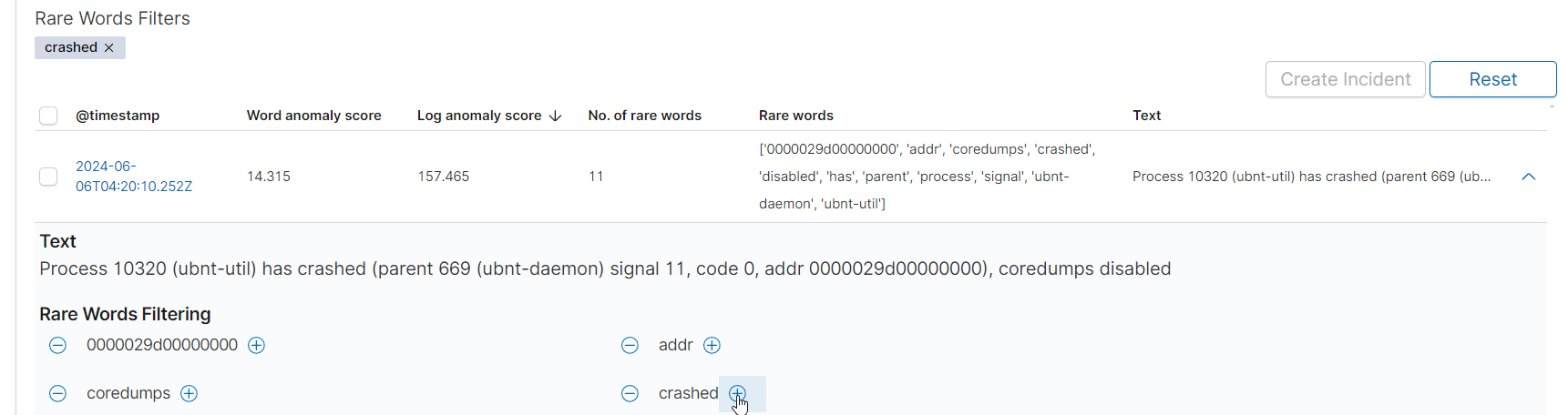../_images/rare_words_filter1.png FilteringRareWords

Actions in the Table¶

Create Incident: A button that allows you to create an incident based on the selected anomaly.
Reset: A button that allows you to reset the filter and refresh the table.

Distinct Anomaly List Table¶

The Distinct Anomaly List tab contains the same anomaly data as the first table but without duplicates. If the message is the same, it is displayed only once. In the first table, all analyzed documents detected as anomalies are displayed, even if one document appears 200 times.

Summary¶

The Performance Tab in Text Anomaly Detection provides key information about detected anomalies. Various charts and tables allow users to visualize anomalies over time, understand their distribution, and review detailed information about each detected anomaly. Correct interpretation of these visualizations is crucial for effectively leveraging anomaly detection capabilities.

Conclusion¶

The Empowered AI module offers comprehensive tools for data analysis, including anomaly detection, clustering, and forecasting. Proper data preparation and rule configuration are crucial for effective analysis. Use the provided guides to leverage the full capabilities of this module.

AI Store¶

The AI Store allows you to download an AI Use Case that matches your index patterns and upload it to your own infrastructure. A short description of each model is available in the drop-down list.

AI Use Case models can be accessed through the Energy Logserver webpage and the Energy Logserver app in the AI Cases => Online Store section.

To upload the selected model through webpage, follow the steps below:

Download the model you are interested in.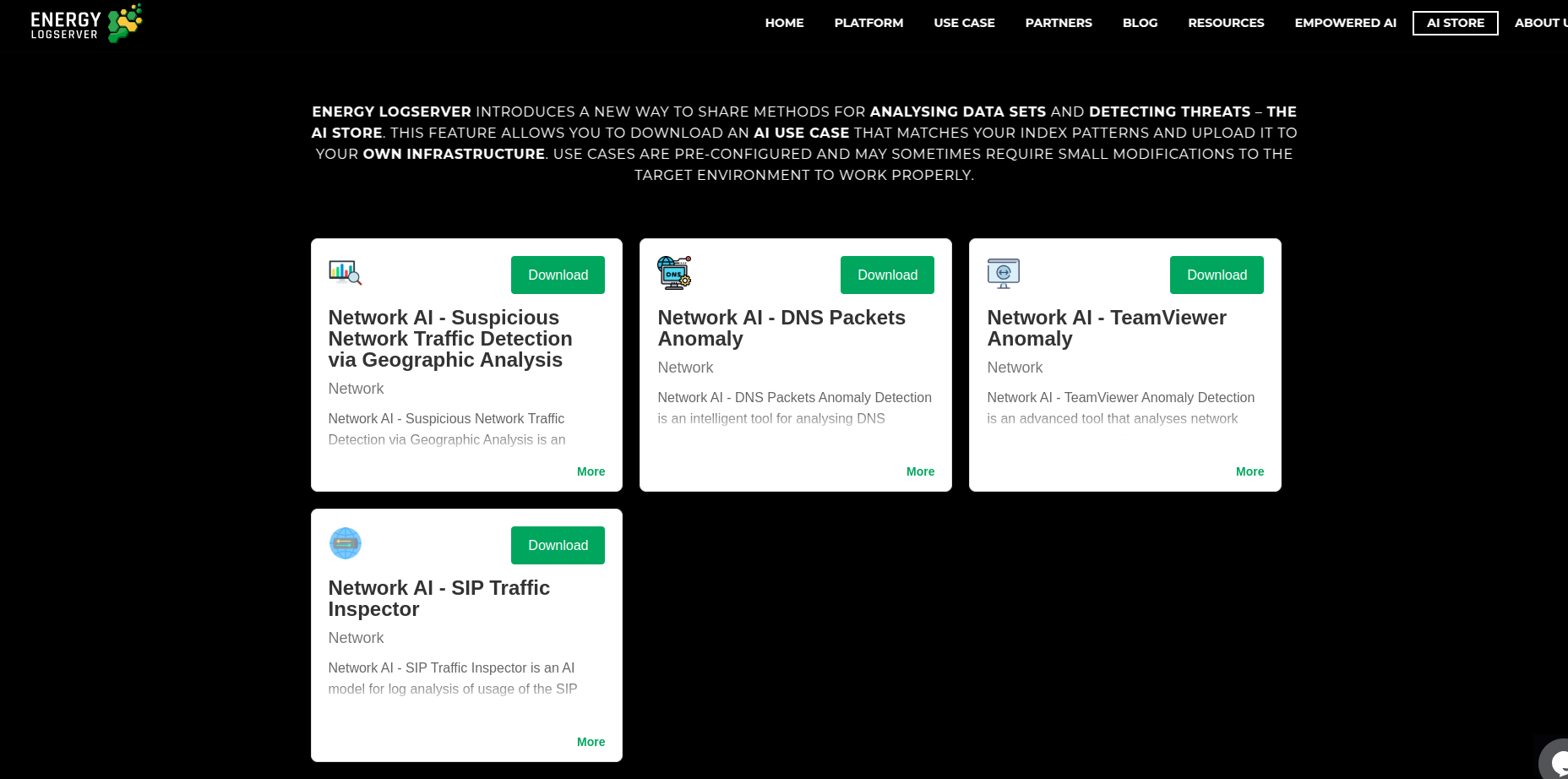
Open the Energy Logserver app and navigate to the AI Cases tab.
Click Upload New Model and select the downloaded model from the file explorer.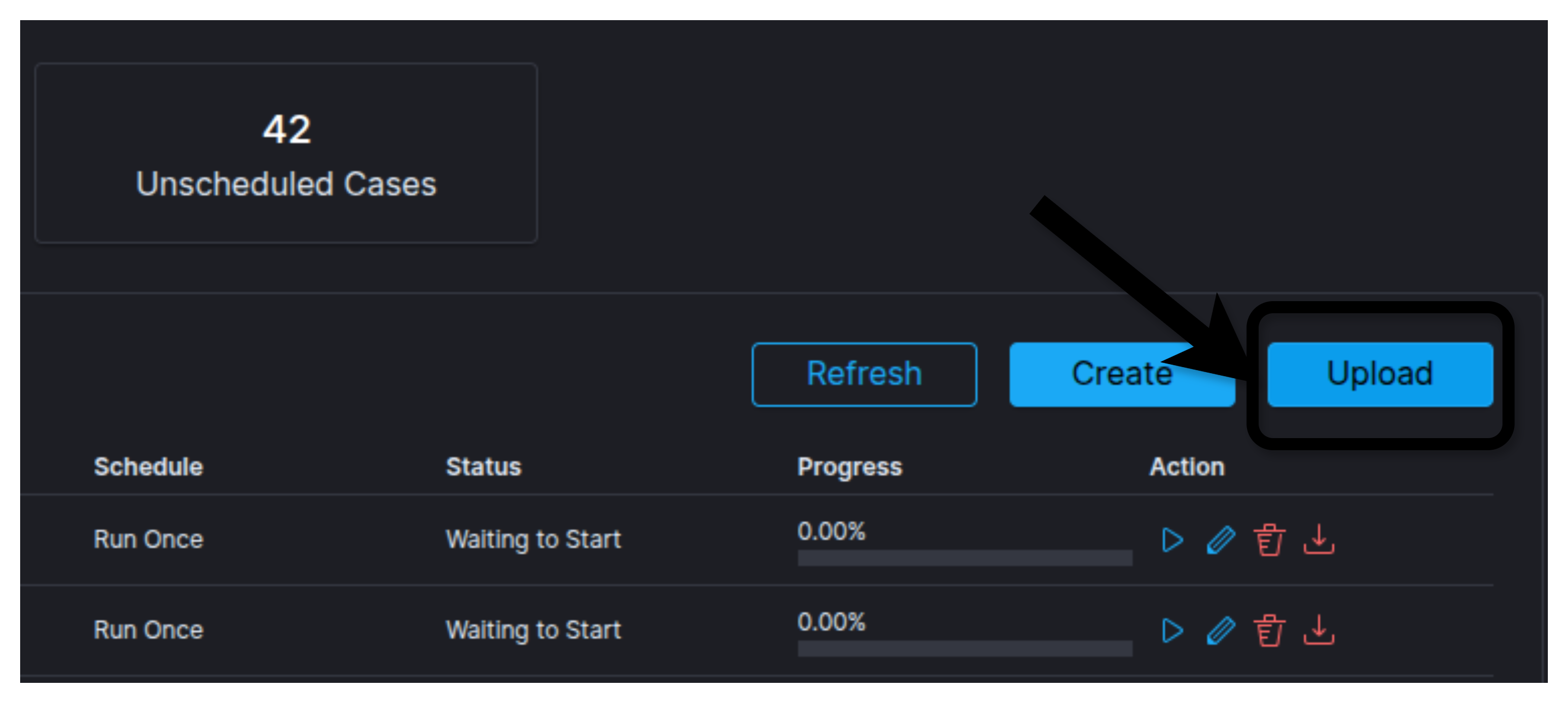
Press Save & Run to start the model.

To upload the selected model via the Energy Logserver app, follow the steps below:

Navigate to AI Cases => Online Store tab.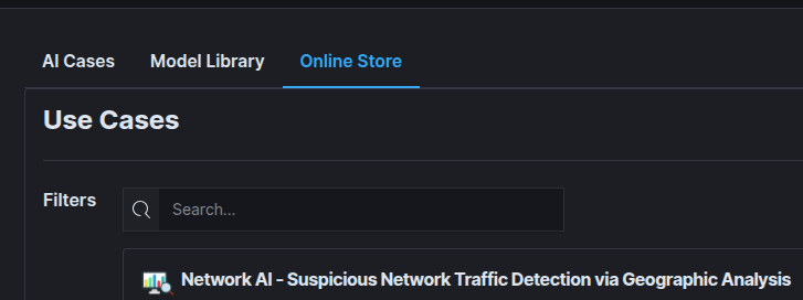
Select the model that you are intrested in and press Fetch button.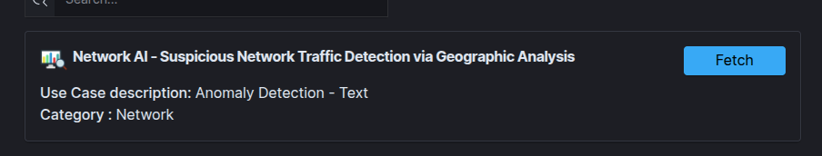
Press Save & Run to start the model.

Default AI Rules¶

Default Rules automatically deploy a set of rules for the syslog index at startup, enabling users to quickly start analyzing data.

Default rules:

Syslog Forecast network.bytes
Syslog Forecast network.ttl
Syslog Forecast postfix_delay
Syslog Forecast postfix_delay_transmission
Syslog Forecast postfix_size
Syslog Forecast count
Syslog Text Anomaly message
Windows-winlogbeat Text Anomaly message
Httpd Text Anomaly message
SIEM-alerts Text Anomaly full_log
SIEM-alerts Text Anomaly data.win.eventdata.data
SIEM-alerts Text Anomaly data.win.system.message
Syslog Univariate network.bytes
Syslog Univariate network.ttl
Syslog Univariate postfix_delay
Syslog Univariate postfix_delay_transmission
Syslog Univariate postfix_size
Syslog Univariate count
Httpd Clustering message
Syslog Clustering message

FAQ¶

Q: What data can I use in saved searches?A: Various types of data can be used, but different analysis models expect specific data types. For example, Text Anomaly detection requires textual values.

Q: Can I edit saved searches?A: Yes, but be cautious as changes affect all rules using the same saved search.

Q: How often should I run the rule?A: The frequency depends on the nature of your data and how often you need to monitor it. For continuous monitoring, consider setting a scheduled analysis at regular intervals.

Q: How many clusters should I choose?A: The number of clusters depends on the nature of your data and the objectives of your analysis. It is recommended to test different values to find the optimal number of clusters for your use case.

Q: What is the purpose of the Data Aggregation setting?A: The Data Aggregation setting defines how data will be grouped over time. It determines the interval at which data points are aggregated.

Q: How do I choose the appropriate Forecast Time Frame?A: The Forecast Time Frame should be selected based on the specific needs of your analysis. Consider the period for which you need the forecast and choose the appropriate time from the available options.

Q: What types of texts in the Text Anomaly use case can be analyzed?A: The system is capable of analyzing various types of textual data, including emails, social media posts, reports, and other textual documents.

Q: Does the system support multiple languages?A: Yes, the text analysis system supports multiple languages, making it a versatile tool on an international scale.

Troubleshooting¶

Problem: I can’t find saved searches in the Empowered AI module.
- Ensure the search is saved in the Discover module and you have the appropriate permissions.
Problem: The rule does not analyze data as expected.
- Check the rule configuration, time range, and search criteria.
Problem: The rule does not detect anomalies as expected.
- Check the contamination factor and data aggregation settings. Adjust these parameters to better fit your data characteristics.
Problem: Too many anomalies are detected.
- Fine-tune the contamination factor to reduce the number of false positives.
Problem: No anomalies are detected despite unusual data patterns.
- Adjust the contamination factor or data aggregation settings to refine the model’s sensitivity.
Problem: Too many anomalies are detected, including normal data variations.
- Fine-tune the contamination factor to reduce the number of false positives.
Problem: Charts do not display data correctly.
- Ensure the data source and configuration settings are correct. Refresh the page or rerun the analysis if necessary.
Problem: Anomaly results appear incorrect.
- Review the contamination factor and other model settings to ensure they are appropriately configured for your data.
Problem: Clustering does not work as expected.
- Check the rule configuration and ensure that all fields are correctly set and that the data is appropriate for clustering.
Problem: I cannot find saved searches in the Empowered AI module.
- Ensure that you have saved the search in the Discover module and that you have the necessary permissions to view it.
Problem: The Cluster Quality Chart does not display correctly.
- Ensure that the data is appropriately prepared and that the clustering rule is correctly configured. Check for errors in the data source or clustering parameters.
Problem: I cannot view clusters in the Discover module.
- Ensure you have the necessary permissions to access the Discover module and that the data is correctly indexed.
Problem: The model’s forecasts do not match the actual data.
- Review the Data Aggregation and Forecast Time Frame settings to ensure they are appropriate for your data. Consider adjusting these settings or re-run the model with different intervals.
Problem: The forecast data does not match the actual data.
- Review the model configuration and ensure that the input data is correct. Check the historical data used to train the model and adjust the model parameters if necessary.
Problem: The system does not analyze the exact number of logs specified.
- Ensure that the number of logs is correctly set and that the available data meets the analysis criteria.
Problem: Delays in text analysis.
- Verify system resources and configuration to increase processing efficiency.
Problem: Incorrect mapping for indices when starting a rule.

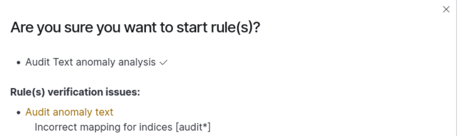StartRuleIndicesMappingWarning
- This indicates that the new mapping required for analysis has not yet been applied. The new mapping will be applied when a new index is created, which occurs on the next day for daily indices (e.g., index_name-2024.03.03) or on the next month for monthly indices (e.g., index_name-2024.03).
Problem: The rule shows ERROR after the run or the results of the analysis are unsatisfactory.
- This probably means that it is necessary to adjust the learning parameters. We recommend the following steps:
1. Press the Edit button
2. Set new Build Time Frame to a period where the data occurs (7 days recommended)
3. Set the new Start Date as the start date of the analysis (we recommend setting this parameter to the day when the Build Time Frame starts).
4. Click Save and Run to start the process.